【書評： 統計学が分かる回帰分析・因子分析編】回帰分析の便利さに触れられます！

この本のシリーズ本の『統計学がわかる』がすごくわかりやすかったので、その続きの本『統計学がわかる 回帰分析・因子分析編』を読みました。

こちらの本もアイスクリーム屋さんの店長と店員を軸に、テンポよく回帰分析を中心に勉強することができます。この本の中で特に参考になった点をピックアップしてマトメていきます！

🎃 第1章：散布図と相関

ポイント

* 散布図はデータの散らばり具合やデータ同士の関係を表す
* 散布図には、正の相関、負の相関、無相関のパターンがある

確認テスト

# 2) 散布図
score <- c(440, 448, 455, 460, 473, 485, 489, 500, 512, 518, 528, 550, 582, 569, 585, 593, 620, 650, 690)< span>seiseki <- c(1.57, 1.83, 2.05, 1.14, 2.73, 1.65, 2.02, 2.98, 1.79, 2.63, 2.08, 2.15, 3.44, 3.05, 3.19, 3.42, 3.87, 3.00, 3.12)< span>plot(score, seiseki)
seiseki <- c(1.57, 1.83, 2.05, 1.14, 2.73, 1.65, 2.02, 2.98, 1.79, 2.63, 2.08, 2.15, 3.44, 3.05, 3.19, 3.42, 3.87, 3.00, 3.12)< span>plot(score, seiseki)
plot(score, seiseki)

# 3) 散布図から読み取れること
#=> 散布図に相関があるように見える

👽 第2章：相関係数

ポイント

相関係数 = 偏差席の平均 / (標準偏差X*標準偏差Y)

確認テスト

# 1) 相関係数
score <- c(440, 448, 455, 460, 473, 485, 489, 500, 512, 518, 528, 550, 582, 569, 585, 593, 620, 650, 690)< span>seiseki <- c(1.57, 1.83, 2.05, 1.14, 2.73, 1.65, 2.02, 2.98, 1.79, 2.63, 2.08, 2.15, 3.44, 3.05, 3.19, 3.42, 3.87, 3.00, 3.12)< span>cor(score, seiseki) #=> 0.7617977# 2) 相関係数から言えること#=> 強い相関がある。入試点数が高い人ほど、成績が高い傾向がある
seiseki <- c(1.57, 1.83, 2.05, 1.14, 2.73, 1.65, 2.02, 2.98, 1.79, 2.63, 2.08, 2.15, 3.44, 3.05, 3.19, 3.42, 3.87, 3.00, 3.12)< span>cor(score, seiseki) #=> 0.7617977# 2) 相関係数から言えること#=> 強い相関がある。入試点数が高い人ほど、成績が高い傾向がある
cor(score, seiseki) #=> 0.7617977

# 2) 相関係数から言えること
#=> 強い相関がある。入試点数が高い人ほど、成績が高い傾向がある

🐰 第3章：無相関検定

確認テスト

# 1) 無作為抽出された場合どのようなことが言えるか？
score <- c(440, 448, 455, 460, 473, 485, 489, 500, 512, 518, 528, 550, 582, 569, 585, 593, 620, 650, 690)< span>seiseki <- c(1.57, 1.83, 2.05, 1.14, 2.73, 1.65, 2.02, 2.98, 1.79, 2.63, 2.08, 2.15, 3.44, 3.05, 3.19, 3.42, 3.87, 3.00, 3.12)< span>cor(score, seiseki) #=> 0.7617977#=> 0.575 < 0.76なので、「母集団の相関係数が0」が棄却。相関がある。# 2) (1)の結果をわかりやすい言葉で説明#=> 入学試験の点数と学業成績の間には偶然ではない何らかの相関がある
seiseki <- c(1.57, 1.83, 2.05, 1.14, 2.73, 1.65, 2.02, 2.98, 1.79, 2.63, 2.08, 2.15, 3.44, 3.05, 3.19, 3.42, 3.87, 3.00, 3.12)< span>cor(score, seiseki) #=> 0.7617977#=> 0.575 < 0.76なので、「母集団の相関係数が0」が棄却。相関がある。# 2) (1)の結果をわかりやすい言葉で説明#=> 入学試験の点数と学業成績の間には偶然ではない何らかの相関がある
cor(score, seiseki) #=> 0.7617977
#=> 0.575 < 0.76なので、「母集団の相関係数が0」が棄却。相関がある。

# 2) (1)の結果をわかりやすい言葉で説明
#=> 入学試験の点数と学業成績の間には偶然ではない何らかの相関がある

😸 第4章：回帰直線

ポイント

データとの差(残差)が最小となるところに引いた線を「回帰直線」と呼ぶ
回帰直線の傾き = 相関係数 * (yの標準偏差/xの標準偏差)
回帰直線のy切片 = yの平均 - (傾き*xの平均)
回帰直線はデータを推測するのに利用される

確認テスト

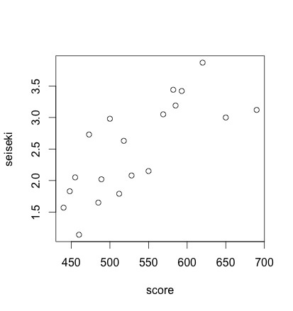
score <- c(440, 448, 455, 460, 473, 485, 489, 500, 512, 518, 528, 550, 582, 569, 585, 593, 620, 650, 690)< span>seiseki <- c(1.57, 1.83, 2.05, 1.14, 2.73, 1.65, 2.02, 2.98, 1.79, 2.63, 2.08, 2.15, 3.44, 3.05, 3.19, 3.42, 3.87, 3.00, 3.12)< span># 1) 回帰直線dat <- data.frame(score, seiseki)< span>result <- glm(seiseki~score, data="dat," family="gaussian)summary(result)# Call:#   glm(formula = seiseki ~ score, family = gaussian, data = dat)# # Deviance Residuals: #   Min        1Q    Median        3Q       Max  # -0.77362  -0.45589   0.01319   0.35065   0.74367  # # Coefficients:#   Estimate Std. Error t value Pr(>|t|)    # (Intercept) -1.797487   0.896221  -2.006 0.061081 .  # score        0.008068   0.001664   4.849 0.000151 ***#   ---#   Signif. codes:  0 ‘***’ 0.001 ‘**’ 0.01 ‘*’ 0.05 ‘.’ 0.1 ‘ ’ 1# # (Dispersion parameter for gaussian family taken to be 0.2577129)# # Null deviance: 10.4396  on 18  degrees of freedom# Residual deviance:  4.3811  on 17  degrees of freedom# AIC: 32.044# # Number of Fisher Scoring iterations: 2#=> 傾きは0.008068、切片は-1.797487# 2) 400、500、600、700点の予測値# 400点 => 0.008068*400 -1.797 #=> 1.4302# 500点 => 0.008068*500 -1.797 #=> 2.2327# 600点 => 0.008068*600 -1.797 #=> 3.0438# 700点 => 0.008068*700 -1.797 #=> 3.8506
seiseki <- c(1.57, 1.83, 2.05, 1.14, 2.73, 1.65, 2.02, 2.98, 1.79, 2.63, 2.08, 2.15, 3.44, 3.05, 3.19, 3.42, 3.87, 3.00, 3.12)< span># 1) 回帰直線dat <- data.frame(score, seiseki)< span>result <- glm(seiseki~score, data="dat," family="gaussian)summary(result)# Call:#   glm(formula = seiseki ~ score, family = gaussian, data = dat)# # Deviance Residuals: #   Min        1Q    Median        3Q       Max  # -0.77362  -0.45589   0.01319   0.35065   0.74367  # # Coefficients:#   Estimate Std. Error t value Pr(>|t|)    # (Intercept) -1.797487   0.896221  -2.006 0.061081 .  # score        0.008068   0.001664   4.849 0.000151 ***#   ---#   Signif. codes:  0 ‘***’ 0.001 ‘**’ 0.01 ‘*’ 0.05 ‘.’ 0.1 ‘ ’ 1# # (Dispersion parameter for gaussian family taken to be 0.2577129)# # Null deviance: 10.4396  on 18  degrees of freedom# Residual deviance:  4.3811  on 17  degrees of freedom# AIC: 32.044# # Number of Fisher Scoring iterations: 2#=> 傾きは0.008068、切片は-1.797487# 2) 400、500、600、700点の予測値# 400点 => 0.008068*400 -1.797 #=> 1.4302# 500点 => 0.008068*500 -1.797 #=> 2.2327# 600点 => 0.008068*600 -1.797 #=> 3.0438# 700点 => 0.008068*700 -1.797 #=> 3.8506

# 1) 回帰直線
dat <- data.frame(score, seiseki)< span>result <- glm(seiseki~score, data="dat," family="gaussian)summary(result)# Call:#   glm(formula = seiseki ~ score, family = gaussian, data = dat)# # Deviance Residuals: #   Min        1Q    Median        3Q       Max  # -0.77362  -0.45589   0.01319   0.35065   0.74367  # # Coefficients:#   Estimate Std. Error t value Pr(>|t|)    # (Intercept) -1.797487   0.896221  -2.006 0.061081 .  # score        0.008068   0.001664   4.849 0.000151 ***#   ---#   Signif. codes:  0 ‘***’ 0.001 ‘**’ 0.01 ‘*’ 0.05 ‘.’ 0.1 ‘ ’ 1# # (Dispersion parameter for gaussian family taken to be 0.2577129)# # Null deviance: 10.4396  on 18  degrees of freedom# Residual deviance:  4.3811  on 17  degrees of freedom# AIC: 32.044# # Number of Fisher Scoring iterations: 2#=> 傾きは0.008068、切片は-1.797487# 2) 400、500、600、700点の予測値# 400点 => 0.008068*400 -1.797 #=> 1.4302# 500点 => 0.008068*500 -1.797 #=> 2.2327# 600点 => 0.008068*600 -1.797 #=> 3.0438# 700点 => 0.008068*700 -1.797 #=> 3.8506
result <- glm(seiseki~score, data="dat," family="gaussian)summary(result)# Call:#   glm(formula = seiseki ~ score, family = gaussian, data = dat)# # Deviance Residuals: #   Min        1Q    Median        3Q       Max  # -0.77362  -0.45589   0.01319   0.35065   0.74367  # # Coefficients:#   Estimate Std. Error t value Pr(>|t|)    # (Intercept) -1.797487   0.896221  -2.006 0.061081 .  # score        0.008068   0.001664   4.849 0.000151 ***#   ---#   Signif. codes:  0 ‘***’ 0.001 ‘**’ 0.01 ‘*’ 0.05 ‘.’ 0.1 ‘ ’ 1# # (Dispersion parameter for gaussian family taken to be 0.2577129)# # Null deviance: 10.4396  on 18  degrees of freedom# Residual deviance:  4.3811  on 17  degrees of freedom# AIC: 32.044# # Number of Fisher Scoring iterations: 2#=> 傾きは0.008068、切片は-1.797487# 2) 400、500、600、700点の予測値# 400点 => 0.008068*400 -1.797 #=> 1.4302# 500点 => 0.008068*500 -1.797 #=> 2.2327# 600点 => 0.008068*600 -1.797 #=> 3.0438# 700点 => 0.008068*700 -1.797 #=> 3.8506
summary(result)
# Call:
#   glm(formula = seiseki ~ score, family = gaussian, data = dat)
# 
# Deviance Residuals: 
#   Min        1Q    Median        3Q       Max  
# -0.77362  -0.45589   0.01319   0.35065   0.74367  
# 
# Coefficients:
#   Estimate Std. Error t value Pr(>|t|)    
# (Intercept) -1.797487   0.896221  -2.006 0.061081 .  
# score        0.008068   0.001664   4.849 0.000151 ***
#   ---
#   Signif. codes:  0 ‘***’ 0.001 ‘**’ 0.01 ‘*’ 0.05 ‘.’ 0.1 ‘ ’ 1
# 
# (Dispersion parameter for gaussian family taken to be 0.2577129)
# 
# Null deviance: 10.4396  on 18  degrees of freedom
# Residual deviance:  4.3811  on 17  degrees of freedom
# AIC: 32.044
# 
# Number of Fisher Scoring iterations: 2
#=> 傾きは0.008068、切片は-1.797487

# 2) 400、500、600、700点の予測値
# 400点 => 0.008068*400 -1.797 #=> 1.4302
# 500点 => 0.008068*500 -1.797 #=> 2.2327
# 600点 => 0.008068*600 -1.797 #=> 3.0438
# 700点 => 0.008068*700 -1.797 #=> 3.8506

🚜 第5章： 偏相関

ポイント

偏相関 => 変数a, b, yが3つあるとき、変数bと変数yの相関から変数aの影響を取り除いたもの
偏相関係数 => (r_by - (r_ay * r_ab))/(sqrt(1-r_ay^2)*sqrt(1-r_ab^2))
偏相関を言い換えると => 第三の変数との残差同士の相関

確認テスト

# 第５章
score <- c(440, 448, 455, 460, 473, 485, 489, 500, 512, 518, 528, 550, 582, 569, 585, 593, 620, 650, 690)< span>seiseki <- c(1.57, 1.83, 2.05, 1.14, 2.73, 1.65, 2.02, 2.98, 1.79, 2.63, 2.08, 2.15, 3.44, 3.05, 3.19, 3.42, 3.87, 3.00, 3.12)< span>hyotei <- c(5.7, 6.8, 6.2, 5.5, 6.0, 7.3, 7.6, 5.6, 6.5, 7.8, 7.5, 8.2, 7.2, 8.8)< span>dat <- data.frame(score, seiseki, hyotei)< span># 1) 各組み合わせの相関係数cor(score, seiseki)  #=> 0.7617977cor(score, hyotei)   #=> 0.6908645cor(seiseki, hyotei) #=> 0.6072251# 2) 偏相関係数 => http://aoki2.si.gunma-u.ac.jp/R/partial-cor.htmlsource("http://aoki2.si.gunma-u.ac.jp/R/src/partial_cor.R", encoding="euc-jp")partial.cor(dat)# Var 1     Var 2     Var 3# Var 1        NA 0.5958705 0.4435168# Var 2 0.5958705        NA 0.1727862# Var 3 0.4435168 0.1727862        NA#=> Var1(score), Var2(seiseki)は、0.5958705# 3) # scoreとseisekiの相関係数は0.762# hyoteiの影響を取り除いた偏相関係数は0.596# hyoteiの影響を取り除いてもscore, seisekiには中程度の相関がある# => 有意水準1%の限界値0.575よりも偏相関係数0.596が大きいので、有意な相関がある
seiseki <- c(1.57, 1.83, 2.05, 1.14, 2.73, 1.65, 2.02, 2.98, 1.79, 2.63, 2.08, 2.15, 3.44, 3.05, 3.19, 3.42, 3.87, 3.00, 3.12)< span>hyotei <- c(5.7, 6.8, 6.2, 5.5, 6.0, 7.3, 7.6, 5.6, 6.5, 7.8, 7.5, 8.2, 7.2, 8.8)< span>dat <- data.frame(score, seiseki, hyotei)< span># 1) 各組み合わせの相関係数cor(score, seiseki)  #=> 0.7617977cor(score, hyotei)   #=> 0.6908645cor(seiseki, hyotei) #=> 0.6072251# 2) 偏相関係数 => http://aoki2.si.gunma-u.ac.jp/R/partial-cor.htmlsource("http://aoki2.si.gunma-u.ac.jp/R/src/partial_cor.R", encoding="euc-jp")partial.cor(dat)# Var 1     Var 2     Var 3# Var 1        NA 0.5958705 0.4435168# Var 2 0.5958705        NA 0.1727862# Var 3 0.4435168 0.1727862        NA#=> Var1(score), Var2(seiseki)は、0.5958705# 3) # scoreとseisekiの相関係数は0.762# hyoteiの影響を取り除いた偏相関係数は0.596# hyoteiの影響を取り除いてもscore, seisekiには中程度の相関がある# => 有意水準1%の限界値0.575よりも偏相関係数0.596が大きいので、有意な相関がある
hyotei <- c(5.7, 6.8, 6.2, 5.5, 6.0, 7.3, 7.6, 5.6, 6.5, 7.8, 7.5, 8.2, 7.2, 8.8)< span>dat <- data.frame(score, seiseki, hyotei)< span># 1) 各組み合わせの相関係数cor(score, seiseki)  #=> 0.7617977cor(score, hyotei)   #=> 0.6908645cor(seiseki, hyotei) #=> 0.6072251# 2) 偏相関係数 => http://aoki2.si.gunma-u.ac.jp/R/partial-cor.htmlsource("http://aoki2.si.gunma-u.ac.jp/R/src/partial_cor.R", encoding="euc-jp")partial.cor(dat)# Var 1     Var 2     Var 3# Var 1        NA 0.5958705 0.4435168# Var 2 0.5958705        NA 0.1727862# Var 3 0.4435168 0.1727862        NA#=> Var1(score), Var2(seiseki)は、0.5958705# 3) # scoreとseisekiの相関係数は0.762# hyoteiの影響を取り除いた偏相関係数は0.596# hyoteiの影響を取り除いてもscore, seisekiには中程度の相関がある# => 有意水準1%の限界値0.575よりも偏相関係数0.596が大きいので、有意な相関がある
dat <- data.frame(score, seiseki, hyotei)< span># 1) 各組み合わせの相関係数cor(score, seiseki)  #=> 0.7617977cor(score, hyotei)   #=> 0.6908645cor(seiseki, hyotei) #=> 0.6072251# 2) 偏相関係数 => http://aoki2.si.gunma-u.ac.jp/R/partial-cor.htmlsource("http://aoki2.si.gunma-u.ac.jp/R/src/partial_cor.R", encoding="euc-jp")partial.cor(dat)# Var 1     Var 2     Var 3# Var 1        NA 0.5958705 0.4435168# Var 2 0.5958705        NA 0.1727862# Var 3 0.4435168 0.1727862        NA#=> Var1(score), Var2(seiseki)は、0.5958705# 3) # scoreとseisekiの相関係数は0.762# hyoteiの影響を取り除いた偏相関係数は0.596# hyoteiの影響を取り除いてもscore, seisekiには中程度の相関がある# => 有意水準1%の限界値0.575よりも偏相関係数0.596が大きいので、有意な相関がある

# 1) 各組み合わせの相関係数
cor(score, seiseki)  #=> 0.7617977
cor(score, hyotei)   #=> 0.6908645
cor(seiseki, hyotei) #=> 0.6072251

# 2) 偏相関係数 => http://aoki2.si.gunma-u.ac.jp/R/partial-cor.html
source("http://aoki2.si.gunma-u.ac.jp/R/src/partial_cor.R", encoding="euc-jp")
partial.cor(dat)
# Var 1     Var 2     Var 3
# Var 1        NA 0.5958705 0.4435168
# Var 2 0.5958705        NA 0.1727862
# Var 3 0.4435168 0.1727862        NA
#=> Var1(score), Var2(seiseki)は、0.5958705

# 3) 
# scoreとseisekiの相関係数は0.762
# hyoteiの影響を取り除いた偏相関係数は0.596
# hyoteiの影響を取り除いてもscore, seisekiには中程度の相関がある
# => 有意水準1%の限界値0.575よりも偏相関係数0.596が大きいので、有意な相関がある

参考リンク

R – 偏相関係数

🍮 第6章：重回帰

ポイント

偏回帰係数 => 偏相関の回帰直線の傾き
単回帰 => 1つの説明変数で独立変数(別の変数)を予測するモデル
重回帰 => 2つ以上の説明変数で独立変数(別の変数)を予測するモデル
重相関係数 => 実測値と重回帰モデルによる予測値の相関関係

確認テスト

score <- c(440, 448, 455, 460, 473, 485, 489, 500, 512, 518, 528, 550, 582, 569, 585, 593, 620, 650, 690)< span>seiseki <- c(1.57, 1.83, 2.05, 1.14, 2.73, 1.65, 2.02, 2.98, 1.79, 2.63, 2.08, 2.15, 3.44, 3.05, 3.19, 3.42, 3.87, 3.00, 3.12)< span>hyotei <- c(5.7, 6.8, 6.2, 5.5, 6.0, 7.3, 7.6, 5.6, 6.5, 7.8, 7.5, 8.2, 7.2, 8.8)< span>dat <- data.frame(score, seiseki, hyotei)< span># 1) 重回帰モデルの式#=> 学業成績 = a*評定平均 + b*入試点数 + c# 2)  重回帰モデルの算出result <- glm(seiseki~score+hyotei, data="dat," family="gaussian)summary(result) # Call:#   glm(formula = seiseki ~ score + hyotei, family = gaussian, data = dat)# # Deviance Residuals: #   Min        1Q    Median        3Q       Max  # -0.69843  -0.36003  -0.05394   0.31981   0.77518  # # Coefficients:#   Estimate Std. Error t value Pr(>|t|)   # (Intercept) -2.094111   1.003309  -2.087  0.05322 . # score        0.006935   0.002337   2.968  0.00907 **#   hyotei       0.128121   0.182587   0.702  0.49295   # ---#   Signif. codes:  0 ‘***’ 0.001 ‘**’ 0.01 ‘*’ 0.05 ‘.’ 0.1 ‘ ’ 1# # (Dispersion parameter for gaussian family taken to be 0.265645)# # Null deviance: 10.4396  on 18  degrees of freedom# Residual deviance:  4.2503  on 16  degrees of freedom# AIC: 33.468# # Number of Fisher Scoring iterations: 2#=> a = 0.006935, b = 0.128121, c = -2.094111# 3) 重相関係数 => http://aoki2.si.gunma-u.ac.jp/R/multiple-cor.htmlsource("http://aoki2.si.gunma-u.ac.jp/R/src/multiple_cor.R", encoding="euc-jp")multiple.cor(dat)# score   seiseki    hyotei # 0.8141785 0.7699771 0.7020678#=> 0.7699771
seiseki <- c(1.57, 1.83, 2.05, 1.14, 2.73, 1.65, 2.02, 2.98, 1.79, 2.63, 2.08, 2.15, 3.44, 3.05, 3.19, 3.42, 3.87, 3.00, 3.12)< span>hyotei <- c(5.7, 6.8, 6.2, 5.5, 6.0, 7.3, 7.6, 5.6, 6.5, 7.8, 7.5, 8.2, 7.2, 8.8)< span>dat <- data.frame(score, seiseki, hyotei)< span># 1) 重回帰モデルの式#=> 学業成績 = a*評定平均 + b*入試点数 + c# 2)  重回帰モデルの算出result <- glm(seiseki~score+hyotei, data="dat," family="gaussian)summary(result) # Call:#   glm(formula = seiseki ~ score + hyotei, family = gaussian, data = dat)# # Deviance Residuals: #   Min        1Q    Median        3Q       Max  # -0.69843  -0.36003  -0.05394   0.31981   0.77518  # # Coefficients:#   Estimate Std. Error t value Pr(>|t|)   # (Intercept) -2.094111   1.003309  -2.087  0.05322 . # score        0.006935   0.002337   2.968  0.00907 **#   hyotei       0.128121   0.182587   0.702  0.49295   # ---#   Signif. codes:  0 ‘***’ 0.001 ‘**’ 0.01 ‘*’ 0.05 ‘.’ 0.1 ‘ ’ 1# # (Dispersion parameter for gaussian family taken to be 0.265645)# # Null deviance: 10.4396  on 18  degrees of freedom# Residual deviance:  4.2503  on 16  degrees of freedom# AIC: 33.468# # Number of Fisher Scoring iterations: 2#=> a = 0.006935, b = 0.128121, c = -2.094111# 3) 重相関係数 => http://aoki2.si.gunma-u.ac.jp/R/multiple-cor.htmlsource("http://aoki2.si.gunma-u.ac.jp/R/src/multiple_cor.R", encoding="euc-jp")multiple.cor(dat)# score   seiseki    hyotei # 0.8141785 0.7699771 0.7020678#=> 0.7699771
hyotei <- c(5.7, 6.8, 6.2, 5.5, 6.0, 7.3, 7.6, 5.6, 6.5, 7.8, 7.5, 8.2, 7.2, 8.8)< span>dat <- data.frame(score, seiseki, hyotei)< span># 1) 重回帰モデルの式#=> 学業成績 = a*評定平均 + b*入試点数 + c# 2)  重回帰モデルの算出result <- glm(seiseki~score+hyotei, data="dat," family="gaussian)summary(result) # Call:#   glm(formula = seiseki ~ score + hyotei, family = gaussian, data = dat)# # Deviance Residuals: #   Min        1Q    Median        3Q       Max  # -0.69843  -0.36003  -0.05394   0.31981   0.77518  # # Coefficients:#   Estimate Std. Error t value Pr(>|t|)   # (Intercept) -2.094111   1.003309  -2.087  0.05322 . # score        0.006935   0.002337   2.968  0.00907 **#   hyotei       0.128121   0.182587   0.702  0.49295   # ---#   Signif. codes:  0 ‘***’ 0.001 ‘**’ 0.01 ‘*’ 0.05 ‘.’ 0.1 ‘ ’ 1# # (Dispersion parameter for gaussian family taken to be 0.265645)# # Null deviance: 10.4396  on 18  degrees of freedom# Residual deviance:  4.2503  on 16  degrees of freedom# AIC: 33.468# # Number of Fisher Scoring iterations: 2#=> a = 0.006935, b = 0.128121, c = -2.094111# 3) 重相関係数 => http://aoki2.si.gunma-u.ac.jp/R/multiple-cor.htmlsource("http://aoki2.si.gunma-u.ac.jp/R/src/multiple_cor.R", encoding="euc-jp")multiple.cor(dat)# score   seiseki    hyotei # 0.8141785 0.7699771 0.7020678#=> 0.7699771
dat <- data.frame(score, seiseki, hyotei)< span># 1) 重回帰モデルの式#=> 学業成績 = a*評定平均 + b*入試点数 + c# 2)  重回帰モデルの算出result <- glm(seiseki~score+hyotei, data="dat," family="gaussian)summary(result) # Call:#   glm(formula = seiseki ~ score + hyotei, family = gaussian, data = dat)# # Deviance Residuals: #   Min        1Q    Median        3Q       Max  # -0.69843  -0.36003  -0.05394   0.31981   0.77518  # # Coefficients:#   Estimate Std. Error t value Pr(>|t|)   # (Intercept) -2.094111   1.003309  -2.087  0.05322 . # score        0.006935   0.002337   2.968  0.00907 **#   hyotei       0.128121   0.182587   0.702  0.49295   # ---#   Signif. codes:  0 ‘***’ 0.001 ‘**’ 0.01 ‘*’ 0.05 ‘.’ 0.1 ‘ ’ 1# # (Dispersion parameter for gaussian family taken to be 0.265645)# # Null deviance: 10.4396  on 18  degrees of freedom# Residual deviance:  4.2503  on 16  degrees of freedom# AIC: 33.468# # Number of Fisher Scoring iterations: 2#=> a = 0.006935, b = 0.128121, c = -2.094111# 3) 重相関係数 => http://aoki2.si.gunma-u.ac.jp/R/multiple-cor.htmlsource("http://aoki2.si.gunma-u.ac.jp/R/src/multiple_cor.R", encoding="euc-jp")multiple.cor(dat)# score   seiseki    hyotei # 0.8141785 0.7699771 0.7020678#=> 0.7699771

# 1) 重回帰モデルの式
#=> 学業成績 = a*評定平均 + b*入試点数 + c

# 2)  重回帰モデルの算出
result <- glm(seiseki~score+hyotei, data="dat," family="gaussian)summary(result) # Call:#   glm(formula = seiseki ~ score + hyotei, family = gaussian, data = dat)# # Deviance Residuals: #   Min        1Q    Median        3Q       Max  # -0.69843  -0.36003  -0.05394   0.31981   0.77518  # # Coefficients:#   Estimate Std. Error t value Pr(>|t|)   # (Intercept) -2.094111   1.003309  -2.087  0.05322 . # score        0.006935   0.002337   2.968  0.00907 **#   hyotei       0.128121   0.182587   0.702  0.49295   # ---#   Signif. codes:  0 ‘***’ 0.001 ‘**’ 0.01 ‘*’ 0.05 ‘.’ 0.1 ‘ ’ 1# # (Dispersion parameter for gaussian family taken to be 0.265645)# # Null deviance: 10.4396  on 18  degrees of freedom# Residual deviance:  4.2503  on 16  degrees of freedom# AIC: 33.468# # Number of Fisher Scoring iterations: 2#=> a = 0.006935, b = 0.128121, c = -2.094111# 3) 重相関係数 => http://aoki2.si.gunma-u.ac.jp/R/multiple-cor.htmlsource("http://aoki2.si.gunma-u.ac.jp/R/src/multiple_cor.R", encoding="euc-jp")multiple.cor(dat)# score   seiseki    hyotei # 0.8141785 0.7699771 0.7020678#=> 0.7699771
summary(result) 
# Call:
#   glm(formula = seiseki ~ score + hyotei, family = gaussian, data = dat)
# 
# Deviance Residuals: 
#   Min        1Q    Median        3Q       Max  
# -0.69843  -0.36003  -0.05394   0.31981   0.77518  
# 
# Coefficients:
#   Estimate Std. Error t value Pr(>|t|)   
# (Intercept) -2.094111   1.003309  -2.087  0.05322 . 
# score        0.006935   0.002337   2.968  0.00907 **
#   hyotei       0.128121   0.182587   0.702  0.49295   
# ---
#   Signif. codes:  0 ‘***’ 0.001 ‘**’ 0.01 ‘*’ 0.05 ‘.’ 0.1 ‘ ’ 1
# 
# (Dispersion parameter for gaussian family taken to be 0.265645)
# 
# Null deviance: 10.4396  on 18  degrees of freedom
# Residual deviance:  4.2503  on 16  degrees of freedom
# AIC: 33.468
# 
# Number of Fisher Scoring iterations: 2
#=> a = 0.006935, b = 0.128121, c = -2.094111

# 3) 重相関係数 => http://aoki2.si.gunma-u.ac.jp/R/multiple-cor.html
source("http://aoki2.si.gunma-u.ac.jp/R/src/multiple_cor.R", encoding="euc-jp")
multiple.cor(dat)
# score   seiseki    hyotei 
# 0.8141785 0.7699771 0.7020678
#=> 0.7699771

Speical Thanks

R – 重相関係数

🏀 第7章：多変量データ

ポイント

多変量データ => 沢山のデータからなる変数
相関行列 => 変数どう押しの相関係数を整理した表

🚕 第8章：因子分析

因子分析 => 多変量データを分析する手法の一つ。多くの観測変数を分析することで、観測変数に影響をあたえる共通要因を求める
因子負荷 => 観測変数に対して共通因子がどれくらいの強さで影響をあたえるかを示したもの
因子得点 => それぞれのケースが、各因子に対してどれくらいの重みを持っているかを計算したもの

🐮 お勧めサイト

R による統計処理

いろんな統計入門系のサイトを見ていると、かなり評判がいいのがこちらのサイト。少しずつこなしたい！

データセット一覧 : DoDStat@d

より複雑なデータ・セットがあるので、いろんな解析の勉強をするときに使ってみたい。

🖥 VULTRおすすめ

「VULTR」はVPSサーバのサービスです。日本にリージョンがあり、最安は512MBで2.5ドル/月($0.004/時間)で借りることができます。4GBメモリでも月20ドルです。 最近はVULTRのヘビーユーザーになので、「ここ」から会員登録してもらえるとサービス開発が捗ります！

📚 おすすめの書籍